Introduction
The early architecture of Uber consisted of a monolithic backend application written in Python that used Postgres for data persistence. Since that time, the architecture of Uber has changed significantly, to a model of microservices and new data platforms. Specifically, in many of the cases where we previously used Postgres, we now use Schemaless, a novel database sharding layer built on top of MySQL. In this article, we’ll explore some of the drawbacks we found with Postgres and explain the decision to build Schemaless and other backend services on top of MySQL.
The Architecture of Postgres
We encountered many Postgres limitations:
- Inefficient architecture for writes
- Inefficient data replication
- Issues with table corruption
- Poor replica MVCC support
- Difficulty upgrading to newer releases
We’ll look at all of these limitations through an analysis of Postgres’s representation of table and index data on disk, especially when compared to the way MySQL represents the same data with its InnoDB storage engine. Note that the analysis that we present here is primarily based on our experience with the somewhat old Postgres 9.2 release series. To our knowledge, the internal architecture that we discuss in this article has not changed significantly in newer Postgres releases, and the basic design of the on-disk representation in 9.2 hasn’t changed significantly since at least the Postgres 8.3 release (now nearly 10 years old).
On-Disk Format
A relational database must perform a few key tasks:
- Provide insert/update/delete capabilities
- Provide capabilities for making schema changes
- Implement a multiversion concurrency control (MVCC) mechanism so that different connections have a transactional view of the data they work with
Considering how all of these features will work together is an essential part of designing how a database represents data on disk.
One of the core design aspects of Postgres is immutable row data. These immutable rows are called “tuples” in Postgres parlance. These tuples are uniquely identified by what Postgres calls a ctid. A ctid conceptually represents the on-disk location (i.e., physical disk offset) for a tuple. Multiple ctids can potentially describe a single row (e.g., when multiple versions of the row exist for MVCC purposes, or when old versions of a row have not yet been reclaimed by the autovacuum process). A collection of organized tuples form a table. Tables themselves have indexes, which are organized as data structures (typically B-trees) that map index fields to a ctid payload.
Typically, these ctids are transparent to users, but knowing how they work helps you understand the on-disk structure of Postgres tables. To see the current ctid for a row, you can add “ctid” to the column list in a WHERE clause:
uber@[local] uber=> SELECT ctid, * FROM my_table LIMIT 1;

-[ RECORD 1 ]--------+------------------------------

ctid                 | (0,1)

...other fields here...
To explain the details of the layout, let’s consider an example of a simple users table. For each user, we have an auto-incrementing user ID primary key, the user’s first and last name, and the user’s birth year. We also define a compound secondary index on the user’s full name (first and last name) and another secondary index on the user’s birth year. The DDL to create such a table might be like this:
CREATE TABLE users ( id SERIAL, first TEXT, last TEXT, birth_year INTEGER, PRIMARY KEY (id) ); CREATE INDEX ix_users_first_last ON users (first, last); CREATE INDEX ix_users_birth_year ON users (birth_year); |
Note the three indexes in this definition: the primary key index plus the two secondary indexes we defined.
For the examples in this article we’ll start with the following data in our table, which consists of a selection of influential historical mathematicians:
| id | first | last | birth_year |
| 1 | Blaise | Pascal | 1623 |
| 2 | Gottfried | Leibniz | 1646 |
| 3 | Emmy | Noether | 1882 |
| 4 | Muhammad | al-Khwārizmī | 780 |
| 5 | Alan | Turing | 1912 |
| 6 | Srinivasa | Ramanujan | 1887 |
| 7 | Ada | Lovelace | 1815 |
| 8 | Henri | Poincaré | 1854 |
As described earlier, each of these rows implicitly has a unique, opaque ctid. Therefore, we can think of the internal representation of the table like this:
| ctid | id | first | last | birth_year |
| A | 1 | Blaise | Pascal | 1623 |
| B | 2 | Gottfried | Leibniz | 1646 |
| C | 3 | Emmy | Noether | 1882 |
| D | 4 | Muhammad | al-Khwārizmī | 780 |
| E | 5 | Alan | Turing | 1912 |
| F | 6 | Srinivasa | Ramanujan | 1887 |
| G | 7 | Ada | Lovelace | 1815 |
| H | 8 | Henri | Poincaré | 1854 |
The primary key index, which maps ids to ctids, is defined like this:
| id | ctid |
| 1 | A |
| 2 | B |
| 3 | C |
| 4 | D |
| 5 | E |
| 6 | F |
| 7 | G |
| 8 | H |
The B-tree is defined on the id field, and each node in the B-tree holds the ctid value. Note that in this case, the order of the fields in the B-tree happens to be the same as the order in the table due to the use of an auto-incrementing id, but this doesn’t necessarily need to be the case.
The secondary indexes look similar; the main difference is that the fields are stored in a different order, as the B-tree must be organized lexicographically. The (first, last) index starts with first names toward the top of the alphabet:
| first | last | ctid |
| Ada | Lovelace | G |
| Alan | Turing | E |
| Blaise | Pascal | A |
| Emmy | Noether | C |
| Gottfried | Leibniz | B |
| Henri | Poincaré | H |
| Muhammad | al-Khwārizmī | D |
| Srinivasa | Ramanujan | F |
Likewise, the birth_year index is clustered in ascending order, like this:
| birth_year | ctid |
| 780 | D |
| 1623 | A |
| 1646 | B |
| 1815 | G |
| 1854 | H |
| 1887 | F |
| 1882 | C |
| 1912 | E |
As you can see, in both of these cases the ctid field in the respective secondary index is not increasing lexicographically, unlike in the case of an auto-incrementing primary key.
Suppose we need to update a record in this table. For instance, let’s say we’re updating the birth year field for another estimate of al-Khwārizmī’s year of birth, 770 CE. As we mentioned earlier, row tuples are immutable. Therefore, to update the record, we add a new tuple to the table. This new tuple has a new opaque ctid, which we’ll call I. Postgres needs to be able to distinguish the new, active tuple at I from the old tuple at D. Internally, Postgres stores within each tuple a version field and pointer to the previous tuple (if there is one). Accordingly, the new structure of the table looks like this:
| ctid | prev | id | first | last | birth_year |
| A | null | 1 | Blaise | Pascal | 1623 |
| B | null | 2 | Gottfried | Leibniz | 1646 |
| C | null | 3 | Emmy | Noether | 1882 |
| D | null | 4 | Muhammad | al-Khwārizmī | 780 |
| E | null | 5 | Alan | Turing | 1912 |
| F | null | 6 | Srinivasa | Ramanujan | 1887 |
| G | null | 7 | Ada | Lovelace | 1815 |
| H | null | 8 | Henri | Poincaré | 1854 |
| I | D | 4 | Muhammad | al-Khwārizmī | 770 |
As long as two versions of the al-Khwārizmī row exist, the indexes must hold entries for both rows. For brevity, we omit the primary key index and show only the secondary indexes here, which look like this:
| first | last | ctid |
| Ada | Lovelace | G |
| Alan | Turing | E |
| Blaise | Pascal | A |
| Emmy | Noether | C |
| Gottfried | Leibniz | B |
| Henri | Poincaré | H |
| Muhammad | al-Khwārizmī | D |
| Muhammad | al-Khwārizmī | I |
| Srinivasa | Ramanujan | F |
| birth_year | ctid |
| 770 | I |
| 780 | D |
| 1623 | A |
| 1646 | B |
| 1815 | G |
| 1854 | H |
| 1887 | F |
| 1882 | C |
| 1912 | E |
We’ve represented the old version in red and the new row version in green. Under the hood, Postgres uses another field holding the row version to determine which tuple is most recent. This added field lets the database determine which row tuple to serve to a transaction that may not be allowed to see the latest row version.
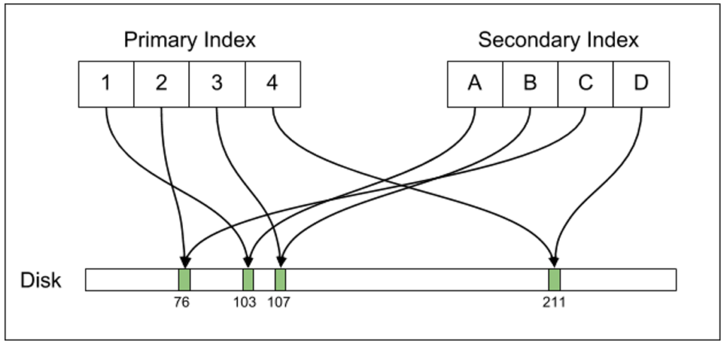
With Postgres, the primary index and secondary indexes all point directly to the on-disk tuple offsets. When a tuple location changes, all indexes must be updated.
Replication
When we insert a new row into a table, Postgres needs to replicate it if streaming replication is enabled. For crash recovery purposes, the database already maintains a write-ahead log (WAL) and uses it to implement two-phase commit. The database must maintain this WAL even when streaming replication is not enabled because the WAL allows the atomicity and durability aspects of ACID.
We can understand the WAL by considering what happens if the database crashes unexpectedly, like during a sudden power loss. The WAL represents a ledger of the changes the database plans to make to the on-disk contents of tables and indexes. When the Postgres daemon first starts up, the process compares the data in this ledger with the actual data on disk. If the ledger contains data that isn’t reflected on disk, the database corrects any tuple or index data to reflect the data indicated by the WAL. It then rolls back any data that appears in the WAL but is from a partially applied transaction (meaning that the transaction was never committed).
Postgres implements streaming replication by sending the WAL on the master database to replicas. Each replica database effectively acts as if it’s in crash recovery, constantly applying WAL updates just as it would if it were starting up after a crash. The only difference between streaming replication and actual crash recovery is that replicas in “hot standby” mode serve read queries while applying the streaming WAL, whereas a Postgres database that’s actually in crash recovery mode typically refuses to serve any queries until the database instance finishes the crash recovery process.
Because the WAL is actually designed for crash recovery purposes, it contains low-level information about the on-disk updates. The content of the WAL is at the level of the actual on-disk representation of row tuples and their disk offsets (i.e., the row ctids). If you pause a Postgres master and replica when the replica is fully caught up, the actual on-disk content on the replica exactly matches what’s on the master byte for byte. Therefore, tools like rsync can fix a corrupted replica if it gets out of date with the master.
Consequences of Postgres’s Design
Postgres’s design resulted in inefficiencies and difficulties for our data at Uber.
Write Amplification
The first problem with Postgres’s design is known in other contexts as write amplification. Typically, write amplification refers to a problem with writing data to SSD disks: a small logical update (say, writing a few bytes) becomes a much larger, costlier update when translated to the physical layer. The same issue arises in Postgres. In our previous example when we made the small logical update to the birth year for al-Khwārizmī, we had to issue at least four physical updates:
- Write the new row tuple to the tablespace
- Update the primary key index to add a record for the new tuple
- Update the (first, last) index to add a record for the new tuple
- Update the birth_year index to add a record for the new tuple
In fact, these four updates only reflect the writes made to the main tablespace; each of these writes needs to be reflected in the WAL as well, so the total number of writes on disk is even larger.
What’s noteworthy here are updates 2 and 3. When we updated the birth year for al-Khwārizmī, we didn’t actually change his primary key, nor did we change his first and last name. However, these indexes still must be updated with the creation of a new row tuple in the database for the row record. For tables with a large number of secondary indexes, these superfluous steps can cause enormous inefficiencies. For instance, if we have a table with a dozen indexes defined on it, an update to a field that is only covered by a single index must be propagated into all 12 indexes to reflect the ctid for the new row.
Replication
This write amplification issue naturally translates into the replication layer as well because replication occurs at the level of on-disk changes. Instead of replicating a small logical record, such as “Change the birth year for ctid D to now be 770,” the database instead writes out WAL entries for all four of the writes we just described, and all four of these WAL entries propagate over the network. Thus, the write amplification problem also translates into a replication amplification problem, and the Postgres replication data stream quickly becomes extremely verbose, potentially occupying a large amount of bandwidth.
In cases where Postgres replication happens purely within a single data center, the replication bandwidth may not be a problem. Modern networking equipment and switches can handle a large amount of bandwidth, and many hosting providers offer free or cheap intra–data center bandwidth. However, when replication must happen between data centers, issues can quickly escalate. For instance, Uber originally used physical servers in a colocation space on the West Coast. For disaster recovery purposes, we added servers in a second East Coast colocation space. In this design we had a master Postgres instance (plus replicas) in our western data center and a set of replicas in the eastern one.
Cascading replication limits the inter–data center bandwidth requirements to the amount of replication required between just the master and a single replica, even if there are many replicas in the second data center. However, the verbosity of the Postgres replication protocol can still cause an overwhelming amount of data for a database that uses a lot of indexes. Purchasing very high bandwidth cross-country links is expensive, and even in cases where money is not an issue it’s simply not possible to get a cross-country networking link with the same bandwidth as a local interconnect. This bandwidth problem also caused issues for us with WAL archival. In addition to sending all of the WAL updates from West Coast to East Coast, we archived all WALs to a file storage web service, both for extra assurance that we could restore data in the event of a disaster and so that archived WALs could bring up new replicas from database snapshots. During peak traffic early on, our bandwidth to the storage web service simply wasn’t fast enough to keep up with the rate at which WALs were being written to it.
Data Corruption
During a routine master database promotion to increase database capacity, we ran into a Postgres 9.2 bug. Replicas followed timeline switches incorrectly, causing some of them to misapply some WAL records. Because of this bug, some records that should have been marked as inactive by the versioning mechanism weren’t actually marked inactive.
The following query illustrates how this bug would affect our users table example:
SELECT * FROM users WHERE id = 4;
This query would return two records: the original al-Khwārizmī row with the 780 CE birth year, plus the new al-Khwārizmī row with the 770 CE birth year. If we were to add ctid to the WHERE list, we would see different ctid values for the two returned records, as one would expect for two distinct row tuples.
This problem was extremely vexing for a few reasons. To start, we couldn’t easily tell how many rows this problem affected. The duplicated results returned from the database caused application logic to fail in a number of cases. We ended up adding defensive programming statements to detect the situation for tables known to have this problem. Because the bug affected all of the servers, the corrupted rows were different on different replica instances, meaning that on one replica row X might be bad and row Y would be good, but on another replica row X might be good and row Y might be bad. In fact, we were unsure about the number of replicas with corrupted data and about whether the problem had affected the master.
From what we could tell, the problem only manifested on a few rows per database, but we were extremely worried that, because replication happens at the physical level, we could end up completely corrupting our database indexes. An essential aspect of B-trees are that they must be periodically rebalanced, and these rebalancing operations can completely change the structure of the tree as sub-trees are moved to new on-disk locations. If the wrong data is moved, this can cause large parts of the tree to become completely invalid.
In the end, we were able to track down the actual bug and use it to determine that the newly promoted master did not have any corrupted rows. We fixed the corruption issue on the replicas by resyncing all of them from a new snapshot of the master, a laborious process; we only had enough capacity to take a few replicas out of the load balancing pool at a time.
The bug we ran into only affected certain releases of Postgres 9.2 and has been fixed for a long time now. However, we still find it worrisome that this class of bug can happen at all. A new version of Postgres could be released at any time that has a bug of this nature, and because of the way replication works, this issue has the potential to spread into all of the databases in a replication hierarchy.
Replica MVCC
Postgres does not have true replica MVCC support. The fact that replicas apply WAL updates results in them having a copy of on-disk data identical to the master at any given point in time. This design poses a problem for Uber.
Postgres needs to maintain a copy of old row versions for MVCC. If a streaming replica has an open transaction, updates to the database are blocked if they affect rows held open by the transaction. In this situation, Postgres pauses the WAL application thread until the transaction has ended. This is problematic if the transaction takes a long amount of time, since the replica can severely lag behind the master. Therefore, Postgres applies a timeout in such situations: if a transaction blocks the WAL application for a set amount of time, Postgres kills that transaction.
This design means that replicas can routinely lag seconds behind master, and therefore it is easy to write code that results in killed transactions. This problem might not be apparent to application developers writing code that obscures where transactions start and end. For instance, say a developer has some code that has to email a receipt to a user. Depending on how it’s written, the code may implicitly have a database transaction that’s held open until after the email finishes sending. While it’s always bad form to let your code hold open database transactions while performing unrelated blocking I/O, the reality is that most engineers are not database experts and may not always understand this problem, especially when using an ORM that obscures low-level details like open transactions.
Postgres Upgrades
Because replication records work at the physical level, it’s not possible to replicate data between different general availability releases of Postgres. A master database running Postgres 9.3 cannot replicate to a replica running Postgres 9.2, nor can a master running 9.2 replicate to a replica running Postgres 9.3.
We followed these steps to upgrade from one Postgres GA release to another:
- Shut down the master database.
- Run a command called pg_upgrade on the master, which updates the master data in place. This can easily take many hours for a large database, and no traffic can be served from the master while this process takes place.
- Start the master again.
- Create a new snapshot of the master. This step completely copies all data from the master, so it also takes many hours for a large database.
- Wipe each replica and restore the new snapshot from the master to the replica.
- Bring each replica back into the replication hierarchy. Wait for the replica to fully catch up to all updates applied by the master while the replica was being restored.
We started out with Postgres 9.1 and successfully completed the upgrade process to move to Postgres 9.2. However, the process took so many hours that we couldn’t afford to do the process again. By the time Postgres 9.3 came out, Uber’s growth increased our dataset substantially, so the upgrade would have been even lengthier. For this reason, our legacy Postgres instances run Postgres 9.2 to this day, even though the current Postgres GA release is 9.5.
If you are running Postgres 9.4 or later, you could use something like pglogical, which implements a logical replication layer for Postgres. Using pglogical, you can replicate data among different Postgres releases, meaning that it’s possible to do an upgrade such as 9.4 to 9.5 without incurring significant downtime. This capability is still problematic because it’s not integrated into the Postgres mainline tree, and pglogical is still not an option for people running on older Postgres releases.
The Architecture of MySQL
In addition to explaining some of Postgres’s limitations, we also explain why MySQL is an important tool for newer Uber Engineering storage projects, such as Schemaless. In many cases, we found MySQL more favorable for our uses. To understand the differences, we examine MySQL’s architecture and how it contrasts with that of Postgres. We specifically analyze how MySQL works with the InnoDB storage engine. Not only do we use InnoDB at Uber; it’s perhaps the most popular MySQL storage engine.
InnoDB On-Disk Representation
Like Postgres, InnoDB supports advanced features like MVCC and mutable data. An exhaustive discussion of InnoDB’s on-disk format is outside the scope of this article; instead, we’ll focus on its core differences from Postgres.
The most important architectural difference is that while Postgres directly maps index records to on-disk locations, InnoDB maintains a secondary structure. Instead of holding a pointer to the on-disk row location (like the ctid does in Postgres), InnoDB secondary index records hold a pointer to the primary key value. Thus, a secondary index in MySQL associates index keys with primary keys:
| first | last | id (primary key) |
| Ada | Lovelace | 7 |
| Alan | Turing | 5 |
| Blaise | Pascal | 1 |
| Emmy | Noether | 3 |
| Gottfried | Leibniz | 2 |
| Henri | Poincaré | 8 |
| Muhammad | al-Khwārizmī | 4 |
| Srinivasa | Ramanujan | 6 |
In order to perform an index lookup on the (first, last) index, we actually need to do two lookups. The first lookup searches the table and finds the primary key for a record. Once the primary key is found, a second lookup searches the primary key index to find the on-disk location for the row.
This design means that InnoDB is at a slight disadvantage to Postgres when doing a secondary key lookup, since two indexes must be searched with InnoDB compared to just one for Postgres. However, because the data is normalized, row updates only need to update index records that are actually changed by the row update. Additionally, InnoDB typically does row updates in place. If old transactions need to reference a row for the purposes of MVCC MySQL copies the old row into a special area called the rollback segment.
Let’s follow what happens when we update al-Khwārizmī’s birth year. If there is space, the birth year field in the row with id 4 is updated in place (in fact, this update always happens in place, as the birth year is an integer that occupies a fixed amount of space). The birth year index is also updated in place to reflect the new date. The old row data is copied to the rollback segment. The primary key index does not need to be updated, nor does the (first, last) name index. If we have a large number of indexes on this table, we still only have to update the indexes that actually index over the birth_year field. So say we have indexes over fields like signup_date, last_login_time, etc. We don’t need to update these indexes, whereas Postgres would have to.
This design also makes vacuuming and compaction more efficient. All of the rows that are eligible to be vacuumed are available directly in the rollback segment. By comparison, the Postgres autovacuum process has to do full table scans to identify deleted rows.
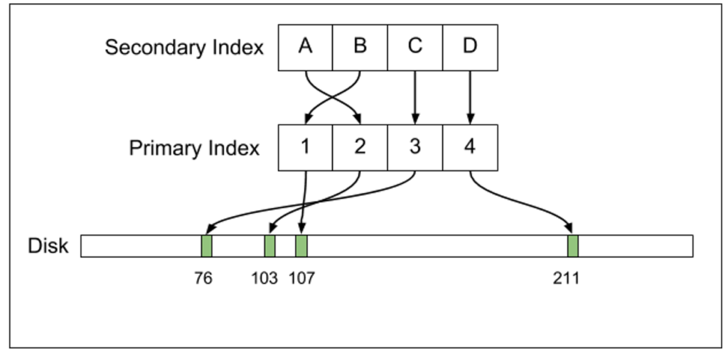
MySQL uses an extra layer of indirection: secondary index records point to primary index records, and the primary index itself holds the on-disk row locations. If a row offset changes, only the primary index needs to be updated.
Replication
MySQL supports multiple different replication modes:
- Statement-based replication replicates logical SQL statements (e.g., it would literally replicate literal statements such as: UPDATE users SET birth_year=770 WHERE id = 4)
- Row-based replication replicates altered row records
- Mixed replication mixes these two modes
There are various tradeoffs to these modes. Statement-based replication is usually the most compact but can require replicas to apply expensive statements to update small amounts of data. On the other hand, row-based replication, akin to the Postgres WAL replication, is more verbose but results in more predictable and efficient updates on the replicas.
In MySQL, only the primary index has a pointer to the on-disk offsets of rows. This has an important consequence when it comes to replication. The MySQL replication stream only needs to contain information about logical updates to rows. The replication updates are of the variety “Change the timestamp for row X from T_1 to T_2.” Replicas automatically infer any index changes that need to be made as the result of these statements.
By contrast, the Postgres replication stream contains physical changes, such as “At disk offset 8,382,491, write bytes XYZ.” With Postgres, every physical change made to the disk needs to be included in the WAL stream. Small logical changes (such as updating a timestamp) necessitate many on-disk changes: Postgres must insert the new tuple and update all indexes to point to that tuple. Thus, many changes will be put into the WAL stream. This design difference means that the MySQL replication binary log is significantly more compact than the PostgreSQL WAL stream.
How each replication stream works also has an important consequence on how MVCC works with replicas. Since the MySQL replication stream has logical updates, replicas can have true MVCC semantics; therefore read queries on replicas won’t block the replication stream. By contrast, the Postgres WAL stream contains physical on-disk changes, so Postgres replicas cannot apply replication updates that conflict with read queries, so they can’t implement MVCC.
MySQL’s replication architecture means that if bugs do cause table corruption, the problem is unlikely to cause a catastrophic failure. Replication happens at the logical layer, so an operation like rebalancing a B-tree can never cause an index to become corrupted. A typical MySQL replication issue is the case of a statement being skipped (or, less frequently, applied twice). This may cause data to be missing or invalid, but it won’t cause a database outage.
Finally, MySQL’s replication architecture makes it trivial to replicate between different MySQL releases. MySQL only increments its version if the replication format changes, which is unusual between various MySQL releases. MySQL’s logical replication format also means that on-disk changes in the storage engine layer do not affect the replication format. The typical way to do a MySQL upgrade is to apply the update to one replica at a time, and once you update all replicas, you promote one of them to become the new master. This can be done with almost zero downtime, and it simplifies keeping MySQL up to date.
Other MySQL Design Advantages
So far, we’ve focused on the on-disk architecture for Postgres and MySQL. Some other important aspects of MySQL’s architecture cause it to perform significantly better than Postgres, as well.
The Buffer Pool
First, caching works differently in the two databases. Postgres allocates some memory for internal caches, but these caches are typically small compared to the total amount of memory on a machine. To increase performance, Postgres allows the kernel to automatically cache recently accessed disk data via the page cache. For instance, our largest Postgres replicas have 768 GB of memory available, but only about 25 GB of that memory is actually RSS memory faulted in by Postgres processes. This leaves more than 700 GB of memory free to the Linux page cache.
The problem with this design is that accessing data via the page cache is actually somewhat expensive compared to accessing RSS memory. To look up data from disk, the Postgres process issues lseek(2) and read(2) system calls to locate the data. Each of these system calls incurs a context switch, which is more expensive than accessing data from main memory. In fact, Postgres isn’t even fully optimized in this regard: Postgres doesn’t make use of the pread(2) system call, which coalesces seek + read operations into a single system call.
By comparison, the InnoDB storage engine implements its own LRU in something it calls the InnoDB buffer pool. This is logically similar to the Linux page cache but implemented in userspace. While significantly more complicated than Postgres’s design, the InnoDB buffer pool design has some huge upsides:
- It makes it possible to implement a custom LRU design. For instance, it’s possible to detect pathological access patterns that would blow out the LRU and prevent them from doing too much damage.
- It results in fewer context switches. Data accessed via the InnoDB buffer pool doesn’t require any user/kernel context switches. The worst case behavior is the occurrence of a TLB miss, which is relatively cheap and can be minimized by using huge pages.
Connection Handling
MySQL implements concurrent connections by spawning a thread-per-connection. This is relatively low overhead; each thread has some memory overhead for stack space, plus some memory allocated on the heap for connection-specific buffers. It’s not uncommon to scale MySQL to 10,000 or so concurrent connections, and in fact we are close to this connection count on some of our MySQL instances today.
Postgres, however, use a process-per-connection design. This is significantly more expensive than a thread-per-connection design for a number of reasons. Forking a new process occupies more memory than spawning a new thread. Additionally, IPC is much more expensive between processes than between threads. Postgres 9.2 uses System V IPC primitives for IPC instead of lightweight futexes when using threads. Futexes are faster than System V IPC because in the common case where the futex is uncontended, there’s no need to make a context switch.
Beside the memory and IPC overhead associated with Postgres’s design, Postgres seems to simply have poor support for handling large connection counts, even when there is sufficient memory available. We’ve had significant problems scaling Postgres past a few hundred active connections. While the documentation is not very specific about why, it does strongly recommend employing an out-of-process connection pooling mechanism to scale to large connection counts with Postgres. Accordingly, using pgbouncer to do connection pooling with Postgres has been generally successful for us. However, we have had occasional application bugs in our backend services that caused them to open more active connections (usually “idle in transaction” connections) than the services ought to be using, and these bugs have caused extended downtimes for us.
Conclusion
Postgres served us well in the early days of Uber, but we ran into significant problems scaling Postgres with our growth. Today, we have some legacy Postgres instances, but the bulk of our databases are either built on top of MySQL (typically using our Schemaless layer) or, in some specialized cases, NoSQL databases like Cassandra. We are generally quite happy with MySQL, and we may have more blog articles in the future explaining some of its more advanced uses at Uber.
Evan Klitzke is a staff software engineer within Uber Engineering‘s core infrastructure group. He is also a database enthusiast and joined Uber as an engineering early bird in September 2012.
- CATEGORIES: Architecture /
- Tags: Data, Database, Infra, MySQL, Open Source, Postgres, Uber Data