I’ve broached the subject of embeddings/embedding vectors in prior blog posts on vector databases and ML application development, but haven’t yet done a deep dive on embeddings and some of the theory behind how embedding models work. As such, this article will be dedicated towards going a bit more in-depth into embeddings/embedding vectors, along with how they are used in modern ML algorithms and pipelines.
A quick note - this article will require an intermediate knowledge of deep learning and neural networks. If you’re not quite there yet, I recommend first taking a look at Google’s ML Crash Course. The course contents are great for understanding the basics of neural networks for CV and NLP.
A quick recap
Vectorizing data via embeddings [1] is, at its heart, a method for dimensionality reduction. Traditional dimensionality reduction methods - PCA, LDA, etc. - use a combination of linear algebra, kernel tricks, and other statistical methods to “compress” data. On the other hand, modern deep learning models perform dimensionality reduction by mapping the input data into a latent space, i.e. a representation of the input data where nearby points correspond to semantically similar data points. What used to be a one-hot vector representing a single word or phrase, for example, can now be represented as a dense vector with a significantly lower dimension. We can see this in action with the Towhee library:
% pip install towhee  # pip3
% python              # python3
>>> import towhee
>>> text_embedding = towhee.dc(['Hello, world!']) \
...     .text_embedding.transformers(model_name='distilbert-base-cased') \
...     .to_list()[0]
...
>>> embedding  # includes punctuation and start & end tokens
array([[ 0.30296388,  0.19200979,  0.10141158, ..., -0.07752968,  0.28487974, -0.06456392],
       [ 0.03644813,  0.03014304,  0.33564508, ...,  0.11048479,  0.51030815, -0.05664057],
       [ 0.29160976,  0.43050566,  0.46974635, ...,  0.22705288, -0.0923526 , -0.04366254],
       [ 0.14108554, -0.00599108,  0.34098792, ...,  0.16725197,  0.10088076, -0.06183652],
       [ 0.35695776,  0.30499873,  0.400652  , ...,  0.20334958,  0.37474275, -0.19292705],
       [ 0.6206475 ,  0.50192136,  0.602711  , ..., -0.03119299,  1.1860386 , -0.6167787 ]], dtype=float32)
Embedding algorithms based on deep neural networks are almost universally considered to be stronger than traditional dimensionality reduction methods. These embeddings are being used more and more frequently in the industry in a variety of applications, e.g. content recommendation, question-answering, chatbots, etc. As we’ll see later, using embeddings to represent images and text within neural networks has also become increasingly popular in recent years.
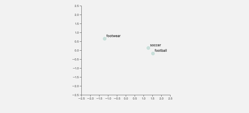 Visualizing text embeddings produced by DistilBERT. Note how "football" is significantly closer to "soccer" than it is to "footwear" despite "foot" being common both words.
Supervised embeddings
So far, my previous articles have used embeddings from models trained using supervised learning, i.e. neural network models which are trained from labelled/annotated datasets. The ImageNet dataset, for example, contains a curated set of image-to-class mappings, while question-answering datasets such as SQuAD provide 1:1 sentence mappings in different languages.
Many well-known models trained across labelled data use cross-entropy loss or mean-squared error. Since the end goal of supervised training is to more or less replicate 1:1 mappings between input data and annotations (e.g. output a class token probability given an input image), embeddings generated from supervised models seldom use the output layer. The standard ResNet50 model trained across ImageNet-1k, for example, outputs a 1000-dimension vector corresponding to probabilities that the input image is an instance of the Nth class label.
 LeNet-5, one of the earliest known neural network architectures for computer vision. Image by D2L.ai, CC BY-SA 4.0.
Instead, most modern applications use the penultimate layer of activations as the embedding. In the image above (LeNet-5), this would correspond to the activations between the layers labelled FC (10) (10-dimensional output layer) and FC (84). This layer is close enough to the output to accurately represent the semantics of the input data while also being a reasonably low dimension. I’ve also seen computer vision applications which use pooled activations from a much earlier layer in the model. These activations capture lower-level features of the input image (corners, edges, blogs, etc…), which can result in improved performance for tasks such as logo recognition.
Encoders and self-supervision
A major downside of using annotated datasets is that they require annotations (this sounds a bit idiotic, but bear with me here). Creating high-quality annotations for a particular set of input data requires hundreds if not thousands of hours of curation by one or many humans. The full ImageNet dataset, for example, contains approximately 22k categories and required an army of 25000 humans to curate. To complicate matters further, many labelled datasets often times contain unintended inaccuracies, flat-out errors, or NSFW content in the curated results. As the number of such instances increases, the quality of embeddings generated by an embedding model trained with supervised learning decreases significantly.
 An image tagged as "Hope" from the Unsplash dataset. To humans, this is a very sensible description, but it may cause a model to learn the wrong types of features during training. Photo by Lukas L.
Models trained in an unsupervised fashion, on the other hand, do not require labels. Given the insane amount of text, images, audio, and video generated on a daily basis, models trained using this method essentially have access to an infinite amount of training data. The trick here is developing the right type of models and training methodologies for leveraging this data. An incredibly powerful and increasing popular way of doing this is via autoencoders (or encoder/decoder architectures in general).
Autoencoders generally have two main components. The first component is an encoder: it takes some piece of data as the input and transforms it into a fixed-length vector. The second component is a decoder: it maps the vector back into the original piece of data. This is known as an encoder-decoder architecture [1]:
 Illustration of encoder-decoder architecture. Image by D2L.ai, CC BY-SA 4.0.
The blue boxes corresponding to the Encoder and Decoder are both feed-forward neural networks, while the State is the desired embedding. There’s nothing paricularly special about either of these networks - many image autoencoders will use a standard ResNet50 or ViT for the encoder network and a similarly large network for the decoder.
Since autoencoders are trained to map the input to a latent state and then back to the original data, unsupervised or self-supervised embeddings are taken directly from the output layer of an encoder as opposed to an intermediate layer for models trained with full supervision. As such, autoencoder embeddings are only meant to be used to for reconstruction [2]. In other words, they can be used to represent the input data but are generally not powerful enough to represent semantics, such as what differentiates a photo of a cat from a photo of a dog.
In recent years, numerous improvements to self-supervision beyond the traditional autoencoder have come about [3]. For NLP, pre-training models with context, i.e. where a word or character appears relative to others in the same sentence or phrase, is commonplace and is now considered the de-facto technique for training state-of-the-art text embedding models [3]. Self-supervised computer vision embedding models are also roaring to life; contrastive training techniques that rely on data augmentation have shown great results when applied to general computer vision tasks. SimCLR and data2vec are two examples of neural networks that make use of masking and/or other augmentations for self-supervised training.
 An Illustration of SimCLR. The "representation" layer in the above illustration corresponds to embeddings generated by a convolutional neural network, i.e. the intermediate state. Image by Google Research.
Embeddings as an input to other models
Embedding models are highly unique; not only are they valuable for generic application development, but their outputs are often used in other machine learning models. Vision transformers are an excellent example of this. Their popularity has exploded in the past two years, aided by strong performance and a large receptive field unavailable to traditional convolutional neural networks. The core premise of vision transformers is to divide an image into square patches, generate embeddings for each patch, and use the embeddings as inputs into a standard transformer. This, surprisingly, works very well for image recognition.
Another great example of this is OpenAI’s CLIP, a large neural network model that is trained to match images with natural language. CLIP is trained on what amounts to essentially infinite data from the internet, e.g. Flickr photos and the corresponding photo title.
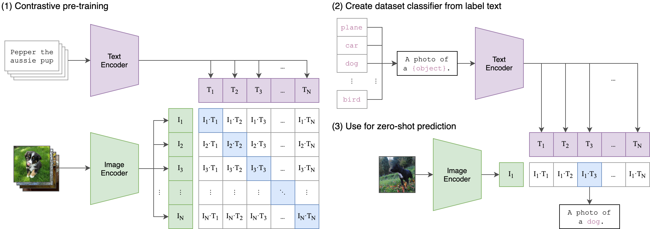 Encoders and their corresponding embeddings are used to great effect in OpenAI's CLIP model. Image by OpenAI, CC BY-SA 4.0.
The methodology behind CLIP is actually fairly straightforward. First, CLIP maps images and text into a latent state (i.e. an embedding); these latent states are then trained to map to the same space, i.e. a text embedding and image embedding should be very close to each other if the text is able to accurately describe the image. The devil is in the details, when it comes to ML, and CLIP is actually fairly difficult to implement in practice without a sizeable dataset and some hyperparameter tuning.
CLIP is used as a core component in DALLE (and DALLE-2), a text-to-image generation engine from OpenAI. There’s been a lot of buzz around DALLE-2 recently, but none of that would be possible without CLIP’s representational power. While CLIP and DALLE’s results have been impressive, image embeddings still have significant room for growth. Certain higher-level semantics such as object count and mathematical operations are still difficult to represent in an image embedding.
Generating your own embeddings
I’ve pointed out the Towhee open-source project a couple of times in the past, showing how it can be used to generate embeddings as well as develop applications that require embeddings. Towhee wraps hundreds of image embedding and classification models from a variety of sources (timm, torchvision, etc…) and that are trained with a variety of different techniques. Towhee also has many NLP models as well, courtesy of 🤗’s Transformers library.
Let’s take a step back and peek at how Towhee generates these embeddings under the hood.
>>> from towhee import pipeline
>>> p = pipeline('image-embedding')
>>> embedding = p('towhee.jpg')
With Towhee, the default method for generating embeddings from a supervised model is simply to remove the final classification or regression layer. For PyTorch models, we can do so with the following example code snippet:
>>> import torch.nn as nn
>>> import torchvision
>>> resnet50 = torchvision.models.resnet50(pretrained=True)
>>> resnet50_emb = nn.Sequential(*(list(resnet50.children())[:-1]))
The last line in the above code snippet recreates a feed-forward network (nn.Sequential) composed of all layers in resnet50 (resnet50.children()) with the exception of the final layer ([:-1]). Intermediate embeddings can also be generated with the same layer removal method. This step is unnecessary for models trained with contrastive/triplet loss or as an autoencoder.
Models based on timm (for CV) and transformers (for NLP) also maintain their own methods which make feature extraction easy:
>>> import numpy as np
>>> from PIL import Image
>>> import timm
>>> image = numpy.array(Image.open('towhee.jpg'))
>>> model = timm.models.resnet50(pretrained=True)
>>> embedding = model.forward_features(img)
>>> from transformers import AutoTokenizer, AutoModel
>>> tokenizer = AutoTokenizer.from_pretrained('bert-base-uncased')
>>> model = AutoModel.from_pretrained('bert-base-uncased')
>>> inputs = tokenizer('Hello, world!', return_tensors='pt')
>>> outputs = model(**inputs)
>>> embedding = outputs.last_hidden_state()
Towhee maintains wrappers for both timm and transformers:
>>> import towhee
>>> text_embedding = towhee.dc(['Hello, world!']) \
...     .text_embedding.transformers(model_name='distilbert-base-cased') \
...     .to_list()[0]  # same as intro example
...
>>> img_embedding = towhee.glob('towhee.jpg') \
...    .image_decode() \
...    .image_embedding.timm(model_name='resnet50') \
...    .to_list()[0]
...
Other resources
I’ve compiled a short and very incomplete list of other great resources on embeddings, if you want to read more or approach the topic from another perspective:
The Milvus documentation provides an overview of embedding vectors (as it relates to storage and vector databases).
OpenAI maintains page on text embeddings that you can check out.
Will Koehrsen provides a great overview of embeddings. It’s a bit dated (2018), but still a great resource.
See how embeddings are being used at Twitter for recommendation.
Reverse image search is one of many applications for embedding vectors. This tutorial demonstrates how to build one in minutes.
If this post was helpful for you, please consider following me on Twitter. In an upcoming post, I’ll provide a brief overview of similarity search and vector indexing algorithms. Stay tuned!
Footnotes
Adapted from D2L.ai. CC BY-SA 4.0 license.
Input reconstruction is a fairly complex problem. For example, generating embeddings that preserve face details in an input photo is a desireable feature, but a “generic” autoencoder would have trouble doing so.
Patches or crops of whole images do techically have context as well. Algorithms and models which understand context are crucial to the subfield of computer vision/graphics known as inpainting. Pre-training techniques for computer vision appliations hasn’t been as successful, but it will likely become more viable in the near future. This 2021 paper shows how masking patches in an autoencoder can be used for pre-training vision transformers.