【论文复现,含代码】Learning to Compare Image Patches via Convolutional Neural Networks
图像匹配问题,历久而弥新。从上个世纪六十年代起,人们开始使用灰度匹配进行匹配,目前,图像匹配的研究重点为图像特征的提取与描述,初始匹配以及精准匹配。目前,深度学习在图像领域正如火如荼,传统的图像匹配问题应该更好的拥抱深度学习。
目前,将深度学习应用在景象匹配方面的论文依然较少,针对为数不多的几篇经典论文,我将尽力去复现这些论文的内容。
这篇博客要复现的是Learning to Compare Image Patches via Convolutional Neural Networks,这里再提供一篇中文论文 卫星影像匹配的深度卷积神经网络方法。这篇中文论文的主要方法也是基于Sergey Zagoruyko的思路做了一些改进,针对具体问题提出了一些改进方法,主要是网络模型对尺度变化的适应性。结合这篇中文论文,对Sergey Zagoruyko的论文进行复现。
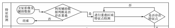
传统的面向结构的影像匹配算法并不能很好地处理异源、多时相及多分辨率卫星影像间的匹配问题。卫星影像相对近景影像,影像目标相对较为单一,内容变化相对简单。本文试图通过深度学习方法,将近年来发展较快的神经网络技术运用到卫星影像特征匹配中,自动学习影像间的匹配模式,实现一种面向对象的卫星影像间自动匹配 流 程,得到更为丰富和更高准确率的匹配点对。
这两篇论文的思路都是搭建一个卷积神经网络,输入两个对应的图像块判断其匹配程度.
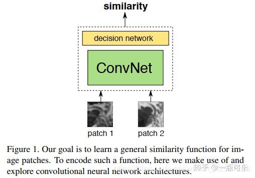
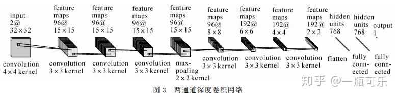
论文中,将两个图像块合并成一个双通道图像,故只需构造一个单通道神经网络,这样使得神经网络的搭建变得十分简单。使用的网络模型如下
下面开始制作样本数据
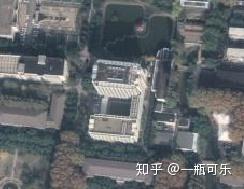
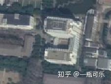
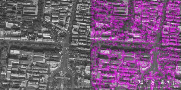
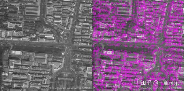
imgPathA = './map/20181123.tif'
imgPathB = './map/20190315.tif'
首先得到两张位置一样的卫星图,分别是2018年与2019年谷歌卫星地图对同一地区的遥感图像。

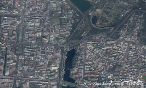
容易发现,这两张图在清晰度和景物上,都存在许多变化,可以很好的应用于遥感图像匹配的样本数据构建中。
景物变化:


拍摄角度变化:


光照阴影变化:
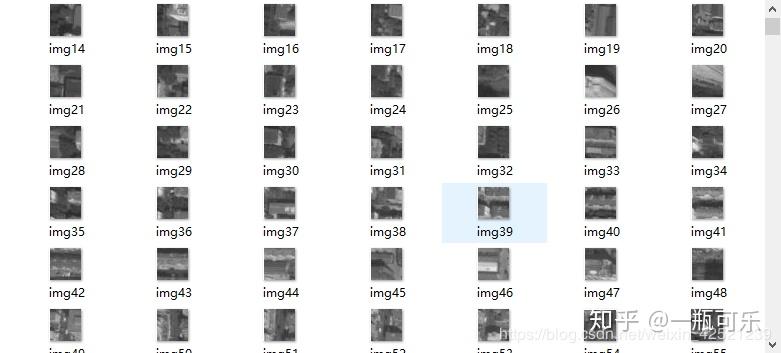
论文中模型的输入为32*32,故依序将两张图片裁剪为32*32的小图片,步长也为32
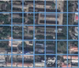
    for i in range(0, imgAsize[1] - 32, 32):
        for j in range(0, imgAsize[0] - 32, 32):
            tempA = imgA[j:(j+32), i:(i+32)]
            tempB = imgB[j:(j+32), i:(i+32)]
            cv2.imwrite("./img/temp/tempA/img" + str(count) + ".jpg", tempA)
            cv2.imwrite("./img/temp/tempB/img" + str(count) + ".jpg", tempB)

            count += 1
分别保存在两个对应的文件夹中并编码
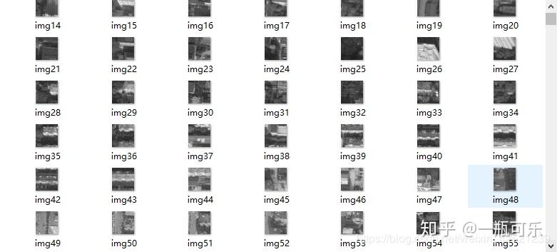
由于两张卫星图都是对同一位置的遥感图像,其像素值对应的坐标是大致相同,由于我们的切分和编码方法也是严格按照顺序来的,所以我们可以直接构造正负样本数据
# 读取文件路径
sampleA = []
for file in os.listdir("./img/temp/tempA"):
sampleA.append("./img/temp/tempA" + "/" + file)
# 读取文件路径
sampleB = []
for file in os.listdir("./img/temp/tempB"):
sampleB.append("./img/temp/tempB" + "/" + file)
tempATrue = cv2.imread(str(sampleTrue[0][i]), 0)
tempBTrue = cv2.imread(str(sampleTrue[1][i]), 0)
cv2.imwrite("./img/true/img" + str(i) + ".jpg",
cv2.merge([tempATrue, tempBTrue, np.zeros([32, 32], dtype="uint8")]))
负样本则是在按顺序排列的基础上,进行随机打乱,那么,两张组合起来的图片在统计学上就是错误匹配的 。
sampleTrue = []
    sampleFalse = []
    sampleTrue = np.array([sampleA, sampleB])
    sampleFalse = np.array([sampleA, sampleB])

    np.random.shuffle(sampleFalse[0])
    np.random.shuffle(sampleFalse[1])


# 合并错误图像,作负样本
        tempAFalse = cv2.imread(str(sampleFalse[0][i]), 0)
        tempBFalse = cv2.imread(str(sampleFalse[1][i]), 0)
        cv2.imwrite("./img/false/img" + str(i) + ".jpg",
                    cv2.merge([tempAFalse, tempBFalse, np.zeros([32, 32], dtype="uint8")]))
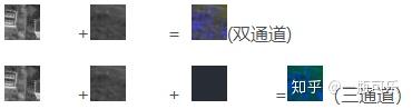
值得一提的是,由于opencv只支持一通道、三通道、四通道图片的保存,因此,在论文双通道的基础之上又叠加了一层全为0的通道图像。即
cv2.merge([tempAFalse, tempBFalse, np.zeros([32, 32], dtype="uint8")])正确样本示意:
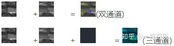
负样本示意:
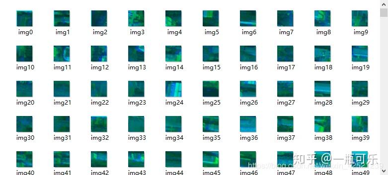
这是制作出的样本数据
由于文中并没有直接给出网络参数,不过可以根据特征图反推回来
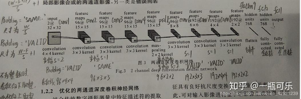
卷积层的部分实现代码如下图所示
# conv1 卷积层1
    with tf.name_scope('conv1') as scope:
        # 卷积核形状为4*4*3,共96个
        kernel = tf.Variable(tf.truncated_normal([4, 4, 3, 96], dtype=tf.float32, stddev=1e-1), name='weights')
        # 输入图像尺寸为32(W)*32*3,padding='VALID'(P),卷积核为4(F)*4*3,步长S=2,输出为(W-F)/S+1=(32-4)/2+1=15 (15*15*96)
        conv = tf.nn.conv2d(img, kernel, [1, 2, 2, 1], padding='VALID')  # 步幅s=2
        biases = tf.Variable(tf.constant(0.0, shape=[96], dtype=tf.float32), trainable=True, name='biases')
        bias = tf.nn.bias_add(conv, biases)
        conv1 = tf.nn.relu(bias, name=scope)

    # conv2 卷积层2
    with tf.name_scope('conv2') as scope:
        # 卷积核形状为3*3*96,共96个
        kernel = tf.Variable(tf.truncated_normal([3, 3, 96, 96], dtype=tf.float32, stddev=1e-1), name='weights')
        # 输入图像尺寸为15(W)*15*96,padding='SAME'(P),卷积核为3(F)*3*96,步长S=1,输出为W/S=15/1=15 (15*15*96)
        conv = tf.nn.conv2d(conv1, kernel, [1, 1, 1, 1], padding='SAME')  # 步幅s=1
        biases = tf.Variable(tf.constant(0.0, shape=[96], dtype=tf.float32), trainable=True, name='biases')
        bias = tf.nn.bias_add(conv, biases)
        conv2 = tf.nn.relu(bias, name=scope)
最后的输出层,网络结构是一个节点,我把他改成了两个,不影响结果,0代表不匹配,1代表匹配。
# flatten9 展开层9
    with tf.name_scope('flatten9') as scope:
        # 将特征图conv8展开为一维,输出为2*2*192=768
        flatten = tf.reshape(conv8, shape=[-1, 2 * 2 * 192])

    # fc10 全连接层10
    with tf.name_scope('fc10') as scope:
        weights = tf.Variable(tf.truncated_normal([768, 768], dtype=tf.float32, stddev=1e-1), name='weights')
        biases = tf.Variable(tf.constant(0.0, shape=[768], dtype=tf.float32), trainable=True, name='biases')
        bias = tf.nn.xw_plus_b(flatten, weights, biases)
        fc10 = tf.nn.relu(bias)

    # fc11 全连接层11
    with tf.name_scope('fc11') as scope:
        weights = tf.Variable(tf.truncated_normal([768, 2], dtype=tf.float32, stddev=1e-1), name='weights')
        biases = tf.Variable(tf.constant(0.0, shape=[2], dtype=tf.float32), trainable=True, name='biases')
        bias = tf.nn.xw_plus_b(flatten, weights, biases)
        fc11 = tf.nn.relu(bias)
接下来定义损失函数
# 损失函数
def losses(logits, label):
    with tf.variable_scope('loss') as scope:  # 让不同命名空间中的变量可以取相同的名字
        cross_entropy = \
            tf.nn.sparse_softmax_cross_entropy_with_logits(logits=logits, labels=label, name="cross_entropy")
        # 得到的是个向量
        loss = tf.reduce_mean(cross_entropy, name='loss')  # 将向量求平均得到loss
    return loss
反向传播算法
# 反向传播算法
def training(loss, learning_rate):
    with tf.name_scope('optimizer'):
        optimizer = tf.train.AdamOptimizer(learning_rate=learning_rate)  # 创建Adam梯度优化器
        global_step = tf.Variable(0, name='global_step', trainable=False)
        train_op = optimizer.minimize(loss, global_step=global_step)  # 对variable变量进行反向优化
    return train_op
评价/准确率计算
# 评价/准确率计算
def evaluation(logits, labels):
    with tf.variable_scope('accuracy') as scope:
        correct = tf.nn.in_top_k(logits, labels, 1)  # 计算预测的结果和实际结果的是否相等,返回一个bool类型的张量
        correct = tf.cast(correct, tf.float16)
        accuracy = tf.reduce_mean(correct)
    return accuracy
训练过程
sess = tf.Session()  # 产生一个会话
saver = tf.train.Saver()  # 产生一个saver来存储训练好的模型
sess.run(tf.global_variables_initializer())  # 所有节点初始化
coord = tf.train.Coordinator()  # 队列监控
threads = tf.train.start_queue_runners(sess=sess, coord=coord)  # 启动队列填充

# 进行batch的训练
try:
    for step in np.arange(MAX_STEP):
        if coord.should_stop():
            break
        _, tra_loss, tra_acc = sess.run([train_op, train_loss, train_acc])

        # 每隔50步打印一次当前的loss以及acc,同时记录log,写入writer
        if step % 10 == 0:
            print('正在训练模型, 当前 Step = %d, 训练进度为 %d %%,train loss = %.2f, train accuracy = %.2f%%' %
                   (step, (step/MAX_STEP)*100, tra_loss, tra_acc * 100.0))
模型训练好之后,基本就没啥问题了。接下来主要是利用一些特征提取算子做一下对比试验。
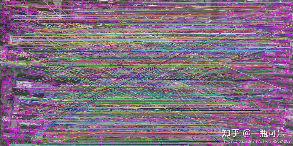
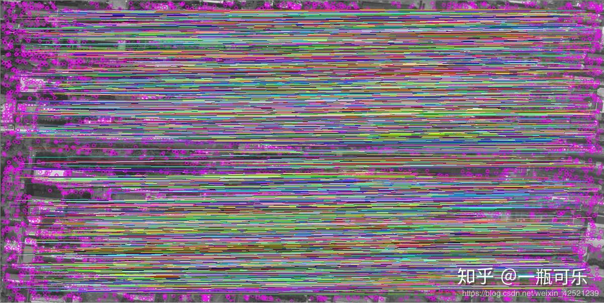
在这儿我主要用了SIFT算子,并用暴力匹配的方法搜索匹配点。
筛选匹配点
good = []
for m, n in matches:
    if m.distance < 0.9*n.distance:
        good.append([m])
匹配点关系如图所示:
在使用深度学习模型进行匹配点的筛选时,依次从图A的特征点中选择一个,然后在图B的特征点中遍历匹配。匹配的方法是,分别在以图A和图B的特征点为中心截取一个32*32的图片,然后输入神经网络,判断是否匹配,如果神经网络的输出为1,则判断这两个特征点是匹配的。
def getImg(x, y, img):
    imgtemp = img[(x-16):(x+16), (y-16):(y+16)]
    return imgtemp
经过深度学习模型筛选后的特征匹配对的连线如下图所示:
可以看到效果是很好的。这也和自己的模型训练的分类正确率有关。
不过在调用模型在筛选匹配点的时候,由于两张图的特征点都比较多,如果做遍历匹配的话速度实在太慢,而论文中也提高了利用辅助数据筛选匹配范围,因此在最后的遍历匹配中,取了特征点左右10个像素浮动做匹配。